The Jacobi Iterative Method

Intro

Concurrent programming began its history in the realm of operating systems but has since found applications in various fields of computer science. Most recently, it has had vast application in the development of machine learning systems.

In computer vision, images are stored as a table of numbers that represent pixel intensities. Furthermore, state of the art computer vision techniques utilize convolutional neural networks (CNNs). These networks are, at the basic level, tables of numbers that represent various features of an image. The process of training CNNs requires efficient computation on those tables. Part of the reason we see the use of GPUs in machine learning development is that they are specialized hardware for such table (matrix) computations.

One of the major efficiency gains in manipulating tables is achieved by dividing up the table into sections and having independent workers (threads) conquer their own sections. As the old saying goes, two heads are better than one. But what about three, or four heads? Gene Amdahl, must have wondered the same thing before he proposed the theoretical limit of parallel computing. He proposed that, the speed up achieved by parallelizing a program is limited by the serial part of the program.

Therefore, parallel computing is most useful for very 'parallelizable' programs. A great example of such a program is known as The Jacobi iterative method. This famous algorithm is used to solve Laplace’s Equation. It iterates over a matrix whose perimeter indices are initialized to some known values. The values in the perimeter could represent measured heat, electrical charge, pressure etc. By averaging the neighboring values of the interior cells (initially unknown) we can find a steady state in which the values in the interior cells are not increasing nor decreasing. This algorithm is a great candidate for parallel computing because different threads, can work on different ‘strips’ of the matrix.

Thread 1 can average the orange section while Thread 2 can work on the blue.

---

Implementation

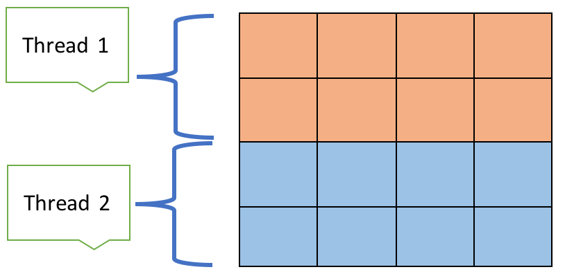
Assume we have t number of execution threads and an n x n matrix we wish to iterate over. Each execution thread can be responsible for (n/t ) x n portion of the matrix. In the figure above, we assume, there are two threads working on two strips of the matrix. In our implementation, thread 1 would be responsible for the top strip of height two. In order for the thread to compute the average value of it’s neighbors, it needs to read the values that thread 2 is responsible for. This highlights a synchronization problem that needs to be addressed. In the implementation adopted from [1]‘Foundations of Multithreaded, Parallel, and Distributed Programming.’ I use two grids and thread barriers to synchronize our threads.

This implementation first reads from our ‘real grid’ and writes the resulting averages to a ‘new grid’. At this point, we need a thread barrier to wait until all threads have completed their computations. This important step, ensures that all cells have their new values, before we do another iteration from the new grid back to the real grid. After we repeat this process we have another thread barrier before we check to see the biggest difference we’ve made among all the cells is a big enough difference. A very small difference -epsilon value- indicates that we are close to a steady state. In this implementation the epsilon value is 0.0001.

---

Java Thread Barrier

This implementation uses the Java programming language. The monitors attached to each object in Java come in convenient in the implementation of thread barriers. It only requires the creation of an object, whose constructor initialized the expected number of threads. Every time a thread calls the ‘awaite’ method of the object this expected number is decremented. We ensure mutual exclusion within this function simply by adding the synchronized key word in the signature of the method. The last thread to call the function releases all awaiting threads and resets the expected number of threads field so the barrier may be reused.

Implementing a thread barrier in Java: NOTH = Number of Threads (Workers)

---

Experiments

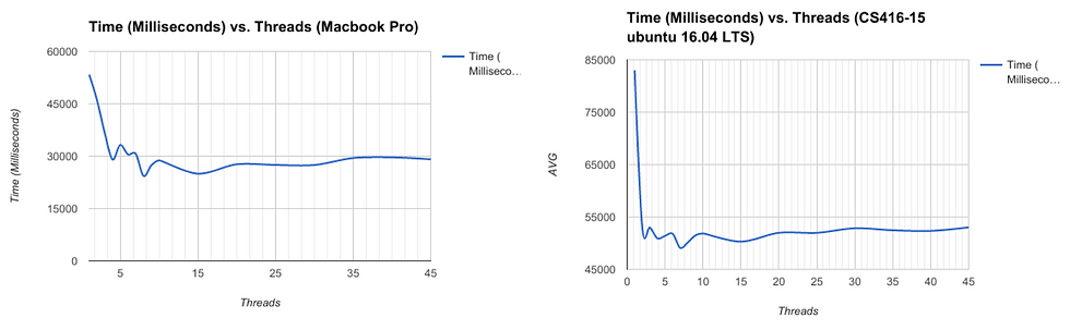
Below is the result of 150 experiments. These were divided up into two machines, a Macbook pro, and a Dell Optiplex(CS405-16). Both these machines have an i7 processor with 4 cores and two threads per core. On each machine, the program ran with 1 to 45 threads

(1,2,3,4,5,6,7,8,9,10,15,20,25,30,35,40, and 45) to be exact. The results are averaged over 5 runs per thread number.

The execution time starte at the creation of the threads, and ended after they are all joined. Considering the inclusion of thread creation, in the experiments, The absolute times are expected to be slightly larger than actual calculation time.

---

Discussion

The program’s performance shows a fairly steady speed up as we utilize more threads. This speed up is however capped at approximately two as depicted in the above figure Also

notable is, that the plateau in the graphs comes after reaching 8 cores. Using anymore than 8 cores does not show any consistent speed up. Furthermore, using as many as 30 or 40 threads shows comparable results to using 8 threads. Comparing this to the theoretical limit proposed by Amdahl’s law, a maximum speed up of two would mean that only 50% of our program is parallelizable.

What we are seeing is theory and practice diverge. The Jacobi algorithm is very parallelizable, but this introduces additional overhead in the form of the barriers.  Is the time spent in the barrier counted toward the serial portion of the code?  Does it count toward the parallel portion?  I would argue toward the serial portion because time spent in the barrier is not making progress toward the solution

There is really another dimension in the experiment.  Varying the size of the matrix would help us better understand the phenomenon.  As the matrix grows in size, the threads stop at the barrier a smaller portion of the time. Therefore we might see more of the performance gains we seek.

These experiments show that the Jacobi iterative method very well illustrates the performance gains of parallel execution. It allows us to use the computing resources we have available to us in an efficient manner. We have also noted that the speed up attained from parallelizing a program does come with some costs. Even though our example and experiments highlighted speed up, it is possible that this speed up diminishes at a higher rate. Considerations such as the rate of memory access, cost of I/O operations pose bottle necks that may not scale as well as adding new processors.

For more on this work please drop me a line at simonyabowerk@gmail.com

The Java implementation can be found at: https://github.com/simonyabo/jacobi

Cheers,

Simon Y. Haile

---

References

[1] R. Andrews, Gregory. (2002). Foundations of Multithreaded, Parallel, and Distributed Programming.